The normal distribution, explained visually
A normal distribution is a symmetric, bell-shaped distribution centered on its mean, μ, with a width set by its standard deviation, σ. About 68% of values lie within one standard deviation of the mean, 95% within two and 99.7% within three. A z-score, z = (x − μ) ÷ σ, counts standard deviations from the mean.
The height of the bell curve at x is 1 divided by σ√(2π), times e raised to the power −(x − μ)² ÷ (2σ²).
Updated
Concept map
8 ideas, in the order to learn them. Click one and Zidna draws and narrates an animated lesson on it.
The Normal Distribution
The normal distribution from the ground up: the bell-shaped pattern it describes, the curve fixed by a mean and a standard deviation, probability as area under it, the 68-95-99.7 rule, z-scores, finding the share of values in any range, and why the bell turns up so often.
Bell-Shaped Data
Data that pile up in one symmetric hump around their average and thin out evenly on both sides, as many measurements do.Generate lesson2Standard Deviation
A measure of spread: roughly how far a typical value lies from the mean, in the same units as the data.Generate lesson3Density Curves
A smooth curve with total area 1 that describes a distribution: the area over any interval is the share of values in it.Generate lesson4The Normal Curve
The symmetric, bell-shaped density curve fixed by two numbers: the mean sets its center and the standard deviation its width.Builds on Bell-Shaped Data, Standard Deviation, Density CurvesGenerate lesson5Z-Scores
The number of standard deviations a value lies above or below the mean: the value minus the mean, divided by the standard deviation.Builds on The Normal CurveGenerate lesson6The 68-95-99.7 Rule
In a normal distribution, about 68%, 95% and 99.7% of values lie within 1, 2 and 3 standard deviations of the mean.Builds on The Normal CurveGenerate lesson7The Central Limit Theorem
The result that sums and averages of many independent random values are close to normal, whatever shape the values themselves have.Builds on The Normal CurveGenerate lesson8Finding Normal Probabilities
Turning a value into a z-score and reading the area under the standard normal curve to find the share of values below, above or between.Builds on The 68-95-99.7 Rule, Z-ScoresGenerate lessonKey ideas
- 01
A normal distribution is fixed by two numbers: the mean μ sets the center of the bell curve and the standard deviation σ sets its width.
- 02
The normal curve is symmetric about its mean, so the mean, median and mode are equal and half of all values lie on each side of the peak.
- 03
In a normal distribution, probability is area: the share of values between two numbers is the area under the curve between them, and the total area is 1.
- 04
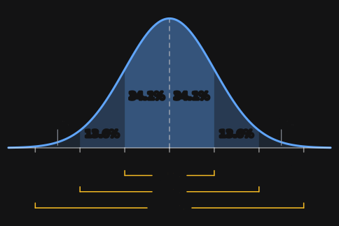
The 68-95-99.7 rule, or empirical rule: about 68% of a normal distribution lies within 1σ of the mean, 95% within 2σ and 99.7% within 3σ.
- 05
A z-score counts standard deviations from the mean: z = (x − μ) ÷ σ. In a normal distribution, a value with z = 2 lies two standard deviations above the mean, higher than about 97.7% of all values.
- 06
Every normal curve has total area 1, so a larger standard deviation makes the bell both wider and lower: doubling σ halves the height of the peak.
What is a normal distribution?
A normal distribution is a continuous probability distribution whose graph is a symmetric, bell-shaped curve. Most values sit near the mean, and values get steadily rarer the farther they are from it, at the same rate on both sides. It is also called the bell curve or the Gaussian distribution.
- Symmetric: the left half of the curve mirrors the right half about the mean, μ.
- One peak, at the mean: the mean, median and mode are all the same number.
- Total area 1: the area under the curve stands for 100% of the values, so the area over any interval is the share of values in it.
- Tails that never touch: the curve gets closer and closer to the horizontal axis without reaching it, so any value is possible, but values far from the mean are very rare.
- Set by two numbers: the mean μ and the standard deviation σ. Two normal distributions with the same μ and σ are identical.
Plenty of real measurements are close to normal: the heights of adults of the same sex, repeated measurements of the same quantity, and scores on tests designed to follow a bell curve, such as IQ tests. A normal distribution is a model, so real data only ever fit it approximately.
How do the mean and standard deviation change the bell curve?
The mean μ slides the bell curve left or right without changing its shape, and the standard deviation σ stretches or squeezes it. A normal distribution with mean μ and standard deviation σ is usually written , with the variance second; some textbooks write , so check which one your course uses.
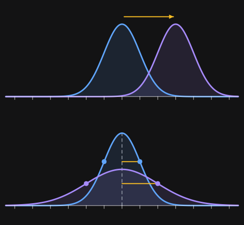
A larger σ makes the curve lower as well as wider. Every normal curve has a total area of 1, so spreading that area over a wider range leaves less height. The peak is , so doubling σ halves it.
To read σ off a graph, find the inflection points: the two places, one on each side of the peak, where the curve stops bending downward and starts bending upward. They sit exactly one standard deviation from the mean, at μ − σ and μ + σ.
The mean is where the bell is centered. The standard deviation is how wide it is, and a wider bell is always a lower one.
What is the 68-95-99.7 rule?
The 68-95-99.7 rule, also called the empirical rule, says that in a normal distribution about 68% of values lie within one standard deviation of the mean, about 95% within two, and about 99.7% within three. It works for every normal distribution, whatever its mean and standard deviation, because every normal curve has the same shape when distance is measured in standard deviations.
| Range | Empirical rule | Exact | Outside the range |
|---|---|---|---|
| μ − σ to μ + σ | 68% | 68.27% | 31.73% |
| μ − 2σ to μ + 2σ | 95% | 95.45% | 4.55% |
| μ − 3σ to μ + 3σ | 99.7% | 99.73% | 0.27% |
The curve is symmetric, so each band splits evenly between the two sides of the mean. The table below gives each band on one side; the other side is the same. When a question says to use the empirical rule, use the numbers in the last column.
| Band | Exact share | By the empirical rule |
|---|---|---|
| μ to μ + σ | 34.13% | 34%, which is 68% ÷ 2 |
| μ + σ to μ + 2σ | 13.59% | 13.5%, which is (95% − 68%) ÷ 2 |
| μ + 2σ to μ + 3σ | 2.14% | 2.35%, which is (99.7% − 95%) ÷ 2 |
| beyond μ + 3σ | 0.13% | 0.15%, which is (100% − 99.7%) ÷ 2 |
- 1Write the mean in the middle of a number line and mark off one standard deviation at a time in both directions.
- 2Find where the values in the question sit on that line.
- 3Add up the bands between them. From the mean out to one side: 34% to μ + σ, 47.5% to μ + 2σ, and 49.85% to μ + 3σ.
- 4For a tail, halve what lies outside the range: above μ + 2σ is (100% − 95%) ÷ 2 = 2.5%.
The 68-95-99.7 rule only holds for data that are close to normal, and only at whole numbers of standard deviations. For any other value, use a z-score and a z-table.
What is a z-score?
A z-score says how many standard deviations a value lies from the mean. Subtract the mean from the value, then divide by the standard deviation:
z equals the value x minus the mean μ, divided by the standard deviation σ.
A positive z-score is above the mean, a negative one is below it, and z = 0 is the mean itself. On a test with mean 70 and standard deviation 8, a score of 82 has : it sits one and a half standard deviations above the mean. To go back from a z-score to a value, reverse the formula: .
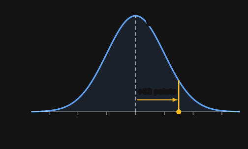
Turning values into z-scores turns every normal distribution into the same one: the standard normal distribution, with mean 0 and standard deviation 1. That is why one table of areas, the z-table, serves heights, test scores and every other normal distribution.
| z-score | Where the value is | Share below (percentile) |
|---|---|---|
| −3 | 3 standard deviations below the mean | 0.13% |
| −2 | 2 standard deviations below the mean | 2.28% |
| −1 | 1 standard deviation below the mean | 15.87% |
| 0 | at the mean | 50% |
| 1 | 1 standard deviation above the mean | 84.13% |
| 2 | 2 standard deviations above the mean | 97.72% |
| 3 | 3 standard deviations above the mean | 99.87% |
How do you find a percentage from a z-score?
The share of values below a z-score is the area under the standard normal curve to the left of it, which a z-table (standard normal table) lists and a calculator gives directly. That share is also the value's percentile. The share above is 1 minus it, and the share between two values is the difference of their two areas.
- 1Turn each value into a z-score: .
- 2Look up the area to the left of each z-score. In a z-table, the row gives z to one decimal place and the column gives the second decimal: for z = 1.25, row 1.2 and column 0.05 give 0.8944.
- 3For the share below a value, that area is the answer: 0.8944, or 89.44%, for z = 1.25.
- 4For the share above, subtract the area from 1: 1 − 0.8944 = 0.1056, or 10.56%.
- 5For the share between two values, subtract the smaller area from the larger one.
| z | 0.00 | 0.01 | 0.02 | 0.03 | 0.04 | 0.05 | 0.06 | 0.07 | 0.08 | 0.09 |
|---|---|---|---|---|---|---|---|---|---|---|
| 1.0 | 0.8413 | 0.8438 | 0.8461 | 0.8485 | 0.8508 | 0.8531 | 0.8554 | 0.8577 | 0.8599 | 0.8621 |
| 1.1 | 0.8643 | 0.8665 | 0.8686 | 0.8708 | 0.8729 | 0.8749 | 0.8770 | 0.8790 | 0.8810 | 0.8830 |
| 1.2 | 0.8849 | 0.8869 | 0.8888 | 0.8907 | 0.8925 | 0.8944 | 0.8962 | 0.8980 | 0.8997 | 0.9015 |
| 1.3 | 0.9032 | 0.9049 | 0.9066 | 0.9082 | 0.9099 | 0.9115 | 0.9131 | 0.9147 | 0.9162 | 0.9177 |
| 1.4 | 0.9192 | 0.9207 | 0.9222 | 0.9236 | 0.9251 | 0.9265 | 0.9279 | 0.9292 | 0.9306 | 0.9319 |
| 1.5 | 0.9332 | 0.9345 | 0.9357 | 0.9370 | 0.9382 | 0.9394 | 0.9406 | 0.9418 | 0.9429 | 0.9441 |
Many z-tables list only positive z-scores. For a negative one, use the symmetry of the curve: the area to the left of −z equals the area to the right of z. The area to the left of z = −1.5 is 1 − 0.9332 = 0.0668.
Most z-tables give the area to the left of z, but some give the area from the mean to z, so check the picture at the top of yours. Below, between and above always add up to 1, which makes a quick check on any answer.
What is the formula for the normal distribution?
The formula for the normal distribution is its probability density function, which gives the height of the bell curve at each value x for a mean μ and a standard deviation σ:
f of x equals 1 over σ times the square root of 2π, times e raised to the power minus (x − μ) squared over 2σ squared.
- The exponent is , where is the z-score. The height depends only on how many standard deviations x is from the mean, which is why every normal curve has the same shape.
- The factor makes the bell. It equals 1 at the mean, where z = 0, and falls fast as z grows: to 0.61 one standard deviation out, 0.14 two out, and 0.011 three out.
- The factor scales the bell so the total area under it is exactly 1.
The height f(x) is a density, not a probability. A probability is the area under the curve between two values, which calculus finds by integrating f(x). That integral has no formula in terms of ordinary functions, so its values come from z-tables and calculators. Because the variable is continuous, the probability of any one exact value is 0.
Why is the normal distribution so common?
A quantity that is the sum or average of many small, independent random effects comes out close to normal, whatever shape each effect has on its own. This is the central limit theorem, and it is why measurement errors, traits shaped by many small causes, and averages of large samples so often follow a bell curve.
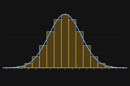
One coin flip gives 0 or 1 head with equal chances: two bars, no bell. The number of heads in 20 flips has mean 20 × 0.5 = 10 and standard deviation √(20 × 0.5 × 0.5) = √5 ≈ 2.24, and its chances follow the normal curve with those values closely. The more independent pieces are added, the closer the fit.
Not every data set is normal. Incomes and house prices, for example, have a long tail to the right, so they are skewed, and the 68-95-99.7 rule does not apply to them.
Worked examples
Using the 68-95-99.7 rule
Scores on an IQ test follow a normal distribution with mean 100 and standard deviation 15. About what percent of people score between 85 and 130, and about what percent score above 130?
- 1Count standard deviations from the mean: is , and is .
- 2From up to the mean is half of 68%: 34%.
- 3From the mean up to is half of 95%: 47.5%.
- 4Between 85 and 130: .
- 5Above 130 is beyond : half of what lies outside two standard deviations, .
Answer: About 81.5% score between 85 and 130, and about 2.5% score above 130. A calculator gives 81.86% and 2.28%, because the rule's numbers are rounded.
Comparing two scores with z-scores
You score 82 on a math test where the mean is 70 and the standard deviation is 8, and 88 on a history test where the mean is 75 and the standard deviation is 10. Which score is better compared with the rest of the class?
- 1Math: .
- 2History: .
- 3Compare the z-scores, not the raw scores: 1.5 standard deviations above the mean beats 1.3.
- 4If both sets of scores are close to normal, the z-table puts the math score above 93.32% of the class and the history score above 90.32%.
Answer: The math score is better relative to its class, against , even though 88 is the higher raw score.
Finding the percentage below, above and between
A machine fills cereal boxes with weights that are normally distributed, with mean 500 g and standard deviation 4 g. What percent of boxes hold less than 494 g, more than 505 g, and between 494 g and 505 g?
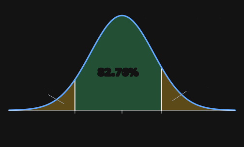
- 1Find the z-scores: and .
- 2Read the areas to the left from a z-table: 0.0668 for and 0.8944 for .
- 3Below 494 g: 0.0668, or 6.68%.
- 4Above 505 g: , or 10.56%.
- 5Between 494 g and 505 g: , or 82.76%. Check: .
Answer: 6.68% of boxes hold less than 494 g, 10.56% hold more than 505 g, and 82.76% hold between 494 g and 505 g. A calculator, which skips the table's rounding, gives 82.75% for the middle.
Finding the score that marks the top 10%
Test scores are normally distributed with mean 72 and standard deviation 9. What score does a student need to be in the top 10%?
- 1The top 10% lies above the cutoff, so 90% lies below it: find the z-score with an area of 0.9000 to its left.
- 2In a z-table, the closest area is 0.8997, in row 1.2 and column 0.08, so .
- 3Turn the z-score back into a score: .
Answer: About 83.5: a score of 84 or more puts a student in the top 10% when the test is scored in whole points.
Check yourself
1.About what percent of a normal distribution lies within 2 standard deviations of the mean?Show answer
About 95% (95.45% to two decimal places).
2.The mean is 50 and the standard deviation is 10. What is the z-score of 65?Show answer
z = (65 − 50) ÷ 10 = 1.5
3.A value has a z-score of −2. Where is it?Show answer
Two standard deviations below the mean.
4.The mean is 100 and the standard deviation is 15. By the 68-95-99.7 rule, about what percent of values are above 115?Show answer
About 16%: 115 is μ + σ, and (100% − 68%) ÷ 2 = 16%.
5.In a normal distribution, how do the mean, median and mode compare?Show answer
They are all equal, at the peak of the curve.
6.The area to the left of z = 1 is 0.8413. What share of values lies above z = 1?Show answer
1 − 0.8413 = 0.1587, about 15.9%
7.Which normal curve has the higher peak: σ = 2 or σ = 5?Show answer
σ = 2. Both have total area 1, so the narrower curve is taller.
8.The mean is 20 and the standard deviation is 4. What value has a z-score of −1.5?Show answer
x = 20 + (−1.5)(4) = 14
Common mistakes
- Reading the height of the curve as a probability.Probability is area under the curve. For a continuous variable, any one exact value has probability 0, and the height can even be more than 1 when σ is small.
- Taking a z-table's number as the share of values above z.Most z-tables give the area to the left of z. For the share above, subtract it from 1.
- Using a "within" percentage for a one-sided question, such as saying 5% of values lie above μ + 2σ.The 5% outside μ ± 2σ is split between the two tails: 2.5% above μ + 2σ and 2.5% below μ − 2σ.
- Reading as a standard deviation of 16.In the usual notation , the second number is the variance, so has . Check whether your course writes the variance or the standard deviation second.
- Subtracting the wrong way round: .Always value minus mean, , so values below the mean get negative z-scores.
- Using the 68-95-99.7 rule on data that are skewed or have two peaks.The rule describes the normal curve. Check that a histogram of the data has one roughly symmetric peak before using it.
Questions students ask
Why is it called a bell curve?
Because its graph looks like the outline of a bell: tall and rounded in the middle, sloping down evenly on both sides and flattening out into long tails. It is also called the Gaussian distribution, after the mathematician Carl Friedrich Gauss, who used it to describe errors in astronomical measurements. A few other distributions are bell-shaped too, but "the bell curve" almost always means the normal one.
Why is it called the normal distribution?
"Normal" here means usual or typical. By the end of the 1800s some writers called it the normal distribution because it was seen as the common pattern for measurements, and around 1900 the statistician Karl Pearson popularized the name. Pearson later regretted it, because it leads people to think every other distribution is abnormal. Skewed data are common and perfectly ordinary; they just follow a different distribution.
Is a normal distribution discrete or continuous?
Continuous. A normally distributed variable can take any real value, so the chance of one exact value is 0 and probabilities come from areas over intervals. Counted data, such as the number of heads in 20 coin flips, are discrete but can still be very close to normal.
Can a normal distribution be skewed?
No. A normal distribution is perfectly symmetric about its mean, so its skewness is 0. Data with a long tail on one side are skewed, so they are not normal, even if they have a single peak.
Can a normal distribution have negative values?
Yes. In theory a normal distribution covers every real number, so negative values always have some probability. For a quantity like height, zero is so many standard deviations below the mean that its probability is effectively 0, and the normal model still works well.
What does a z-score of 2 mean, and is it unusual?
A z-score of 2 means the value is two standard deviations above the mean, higher than about 97.7% of a normal distribution. Only about 4.6% of values lie more than two standard deviations from the mean in either direction, so a z-score beyond ±2 is often called unusual, and one beyond ±3, which happens to 0.27% of values, very rare.
What is the difference between a normal and a standard normal distribution?
The standard normal distribution is the normal distribution with mean 0 and standard deviation 1, usually called Z. Any normal distribution becomes it when each value is replaced by its z-score, which is why a single z-table works for every normal distribution.
Why is 1.96 used instead of 2 for 95%?
The 68-95-99.7 rule rounds. Exactly 95% of a normal distribution lies within 1.96 standard deviations of the mean, while 2 standard deviations hold 95.45%. That is where the 1.96 in 95% confidence intervals comes from.
How do you find normal probabilities on a calculator?
On a TI-83 or TI-84, normalcdf(lower, upper, μ, σ) gives the area between two values; use −1E99 or 1E99 for a side with no limit. invNorm(area, μ, σ) works backward from the area to the left of a value to the value itself. In Excel or Google Sheets, NORM.DIST(x, μ, σ, TRUE) gives the area to the left of x.
Does the empirical rule work for any data set?
No. The 68-95-99.7 rule describes normal distributions, and roughly bell-shaped data. For any distribution at all, Chebyshev's inequality guarantees only that at least 75% of values lie within 2 standard deviations of the mean and at least 88.9% within 3.
Is IQ normally distributed?
IQ scores are designed to be. Most modern IQ tests convert raw scores so that, in the group the test was standardized on, they follow a normal distribution with mean 100 and standard deviation 15. So about 68% of that group scores between 85 and 115, and about 95% between 70 and 130.
Sources
Keep going
All math topicsStatistics
Standard deviation, explained visually
Standard deviation measures how spread out numbers are: roughly, how far a typical value sits from the mean. Square each value's distance from the mean, average the squares, then take the square root. For 4, 6, 7, 8 and 10 the mean is 7 and the standard deviation is 2. For a sample, divide by n − 1 instead of n.
Calculus
How to find the area under a curve
The area under y = f(x) from x = a to x = b is the definite integral of f from a to b, the limit of sums of ever-thinner rectangles. It equals F(b) − F(a), where F is an antiderivative of f. For y = x² from 0 to 2, F(x) = x³/3, so the area is 8/3 ≈ 2.67. The integral counts area below the x-axis as negative.